Probability Theory

POLI_SCI 403: Probability and Statistics

Agenda

1. Why do we need probability?

2. Probability theory \(\Rightarrow\) random variables

3. Peek at Lab 1

Why is probability theory important?

You are not allowed to conduct statistical inference unless you are willing to entertain uncertainty in data generation processes

Probability is the language of uncertainty (random events)

But nothing is actually random

Probability theory is a mathematical construct

Why is probability theory important?

You are not allowed to conduct statistical inference unless you are willing to entertain uncertainty in data generation processes

Probability is the language of uncertainty (random events)

But nothing is actually random

Probability theory is a mathematical construct (that supports other, more important, equally shaky mathematical constructs)

Probability is a modeling assumption

Probability is a modeling assumption

And yet, any numerical probability… is not an objective property of the world, but a construction based on personal or collective judgements and (often doubtful) assumptions. Furthermore, in most circumstances, it is not even estimating some underlying ‘true’ quantity. Probability, indeed, can only rarely be said to ‘exist’ at all.

Probability is a modeling assumption

“…it handles both chance and ignorance.”

“…any practical use of probability involves subjective judgements.”

Events are uncertain only because we cannot measure with arbitrary precision

Examples

What is the probability of landing heads when flipping an unbiased coin?

What is the probability of rolling or with a fair dice?

What about a biased coin? An unfair die?

Why do we need such language?

 

We are making the problem tractable so that the answer can be something other than “I don’t know”

A more involved example
(Stark and Freedman)

What is the chance that an earthquake of magnitude 6.7 or greater will occur before the year 2023?

 

How do we make this tractable?

Approaches to probability

• Symmetry: If outcomes are judged equally likely, then each must have equal probability

• Frequentist: Relative frequency with which the event occurs in repeated trials under the same conditions

• Bayesian: Probability as degree of belief (0: impossible; 1: sure to happen)

Approaches to probability

• Symmetry: If outcomes are judged equally likely, then each must have equal probability

• Frequentist: Relative frequency with which the event occurs in repeated trials under the same conditions

• Bayesian: Probability as degree of belief (0: impossible; 1: sure to happen)

Laplace’s principle of insufficient reason: If there is no reason to believe that outcomes are not equally likely, take them to be equally likely

Approaches to probability

• Symmetry: If outcomes are judged equally likely, then each must have equal probability

• Frequentist: Relative frequency with which the event occurs in repeated trials under the same conditions

• Bayesian: Probability as degree of belief (0: impossible; 1: sure to happen)

Symmetry will be useful when we move to statistical inference proper. Doesn’t make sense for earthquakes

Approaches to probability

• Symmetry: If outcomes are judged equally likely, then each must have equal probability

• Frequentist: Relative frequency with which the event occurs in repeated trials under the same conditions

• Bayesian: Probability as degree of belief (0: impossible; 1: sure to happen)

Frequentist statistics will be the default approach in the methods sequence, but it’s hard to imagine repeating 2000-2030

Approaches to probability

• Symmetry: If outcomes are judged equally likely, then each must have equal probability

• Frequentist: Relative frequency with which the event occurs in repeated trials under the same conditions

• Bayesian: Probability as degree of belief (0: impossible; 1: sure to happen)

Bottomline: Probability does not always make sense

We won’t talk much about Bayesian statistics, but Bayes theorem is very important. Still, for this problem, the Bayesian approach changes the question toward expert opinions

But it does sometimes

Symmetry makes sense when thinking about quasi-experiments

Frequentism makes sense for weather forecasts and is the basis for random sampling and assignment

Bayes makes a lot of sense for latent variables (e.g. ideal point estimation \(\rightarrow\) item-response theory)

What’s the point?

Everything that follows from today is fake

Or, rather, it is held together by a series of heroic, implausible assumptions

And I find that both beautiful AND stupid

But, more importantly, I want you to remember that we use statistical models not because they are true, but because they are useful

So the question about the appropriate method will always be subjective

Probability Theory

Setup

1. \(\Omega\): sample space

\[ \Omega = \{1, 2, 3, 4, 5, 6\} \]

\[ \Omega = \{H,T\} \]

Sample space: Set of all possible outcomes of a random generative process

Setup

1. \(\Omega\): sample space

\[ \Omega = \{1, 2, 3, 4, 5, 6\} \]

\[ \Omega = \{H,T\} \]

\(\omega \in \Omega\) sampling points

Sampling points are individual outcomes in the sampling space

Setup

1. \(\Omega\): sample space

2. \(S \subseteq \Omega\): event space

\[ A = \omega \in \Omega \colon \omega \text{ is even} = \{2,4,6\} \]

Event spaces or just events are subsets of the sample space

Setup

1. \(\Omega\): sample space

2. \(S \subseteq \Omega\): event space

\(S\) is an event space if

• Non-empty: \(S \neq \emptyset\)
• Closed under complements: if \(A \in S\), then \(A^c \in S\)
• Closed under unions:
  if \(A_1, A_2, A_3 \ldots \in S\), then \(A_1 \cup A_2 \cup A_3 \ldots \in S\)

This definition ensures events will have well-defined probabilities

Setup

1. \(\Omega\): sample space

2. \(S \subseteq \Omega\): event space

3. \(P:S \rightarrow \mathbb{R}\): probability measure

These are the basic components required to describe a random generative process

Probability measure: A function that assigns a probability to every event in the event space

Kolmogorov probability axioms

• Non-negativity: \(\forall A \in S, P(A) \geq 0\)
• Unitarity: \(P(\Omega) = 1\)
• Countable additivity: If \(A_1, A_2, A_3, \ldots \in S\) are pairwise disjoint then \(P(A_1 \cup A_2 \cup A_3 \cup \ldots) = \sum_iP(A_i)\)

We are ruling out nonsensical probabilities

Basic properties

• Monotonicity: If \(A \subseteq B\), then \(P(A) \leq P(B)\)
• Subtraction rule: If \(A \subseteq B\), then \(P(B \backslash A) = P(B) - P(A)\)
• Empty set: \(P(\emptyset = 0)\)
• Probability bounds: \(0 \leq P(A) \leq 1\)
• Complement rule: \(P(A^c) = 1-P(A)\)

Monotonicity, bounds, and complement are very important!

Joint and conditional probabilities

• Joint: \(P(A\cap B)\)
• Addition: \(P(A \cup B) = P(A) + P(B) - P(A \cap B)\)
• Conditional: \(P(A|B) = \frac{P(A \cap B)}{P(B)}\)

These make more sense in practice, we cover them in the lab

Independence

Events \(A\) and \(B\) are independent iff

\[ P(A \cap B) = P(A) P(B) \]

Applying the definition of conditional probabilities (or multiplicative law)

\(A\) and \(B\) are independent iff

\[ P(A|B) = P(A) \]

Independence is a core concept in statistics. These are two ways to think about it

Moving on

We now have a language to talk about random generative processes

The next step is to describe or characterize these processes

Random variables

• \(X\) is a random variable.

• A random variable is a function such that \(X:\Omega \rightarrow \mathbb{R}\)

• A mapping of possible states of the world into a real number

• Neither random nor a variable

• Informally: A variable that takes a value determined by a random generative process

• Except that it never takes an actual value

This is weird by construction. We use random variables as a placeholder to think about the properties of random generative processes without actually looking at them. Things will make more sense over the next two weeks.

Random variables are functions

But we can also apply functions to them (e.g. \(g(X) = X^2\))

A (well-behaved) function of a random variable is also a random variable

We can also operate on them (e.g. \(E[X]\) or \(Pr[X = 1]\))

Because we can “do” things to them, we can also describe them

Types of random variables

1. Discrete

2. Continuous

Discrete random variables

\(X\) is discrete if its range \(X(\Omega)\) is a countable set

We can fully characterize the distribution of \(X\) with a Probability Mass Function (PMF)

\[ f(x) = Pr[X = x] \]

This is useful because we can talk about more general cases

I am skipping the condition \(\forall x \in\mathbb{R}\) throughout

Example: Biased coin flip

\[ f(x) =\begin{cases} 1-p & \colon & x = 0 \\ p & : & x = 1 \\ 0 & : & \text{otherwise} \end{cases} \]

Where \(p\) is the expected proportion of tails

This is a Bernoulli distribution

Which is a special case of a binomial distribution

PMFs are usually expressed as cases because probabilities are mapped to each discrete value.

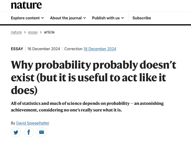
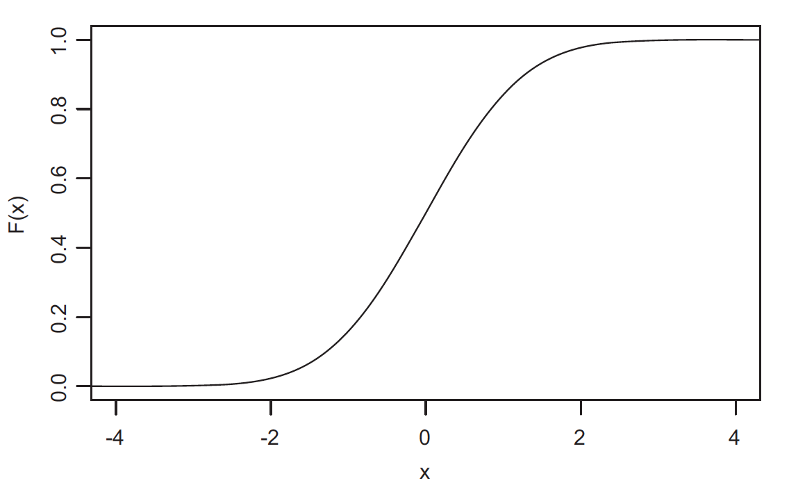
Cumulative distribution function (CDF)

\[ F(x) = Pr[X \leq x] \]

Returns the probability of \(X\) being greater or equal than \(x\)

This is a more general (and more informative) way to describe a random variable

Example: Die roll CDF

Continuous random variables

Informally, a random variable is continuous if its range can be measured to an arbitrary degree of precision

Because working with continuous functions is messier, the definition is recursive

Continuous random variable

\(X\) is a continuous random variable if there exists a non-negative function \(f: \mathbb{R} \to \mathbb{R}\) such that the CDF of X is an integral

\[ F(x) = Pr[X \leq x] = \int_{-\infty}^x f(u)du \]

Meaning the only way we can tell if a random variable is continuous is because its CDF is also continuous

Continuous random variable

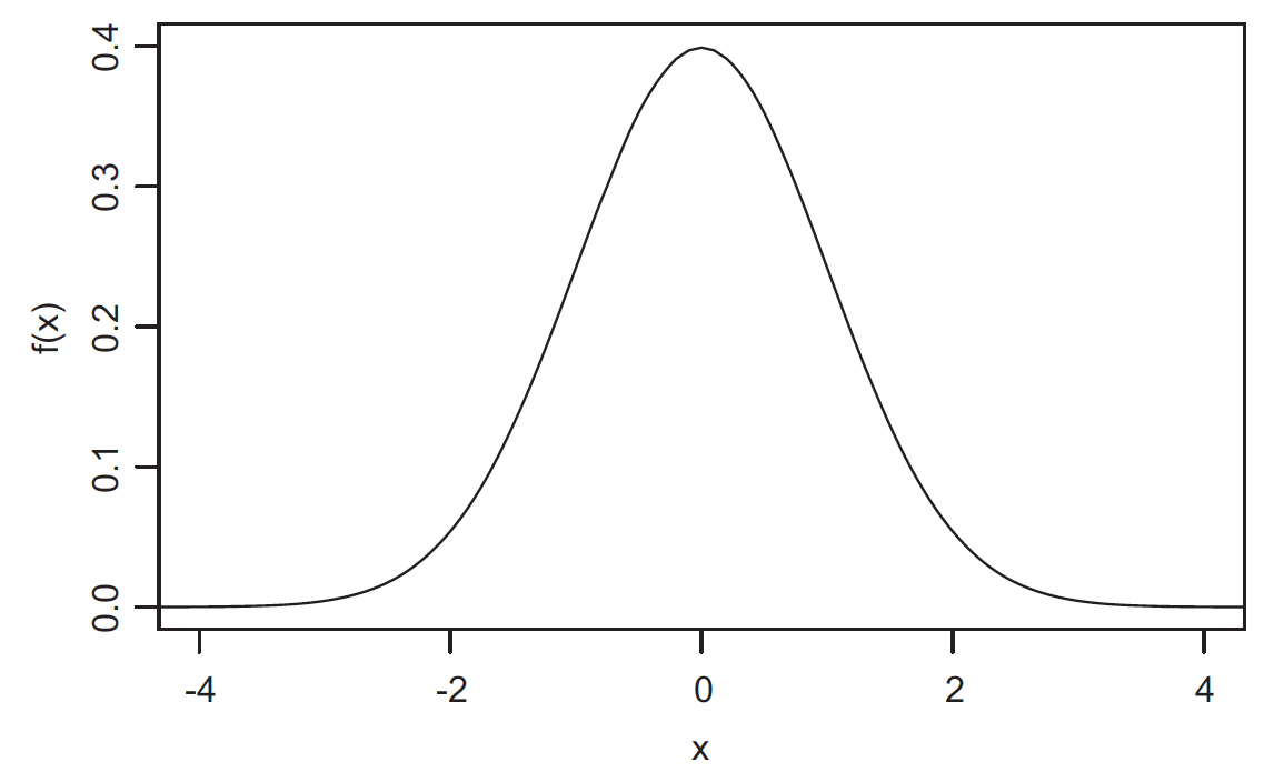
This turns out to be convenient, because the Probability Density Function of a continuous random variable is a derivative

\[ f(x) = \frac{dF(u)}{du} \bigg\rvert_{u=x} \]

So the PDF gives the slope or rate of change at \(x\)

\(\neq\) the PMF of a discrete RV giving the probability exactly at \(x\)

Continuous random variable

This turns out to be convenient, because the Probability Density Function of a continuous random variable is a derivative

\[ f(x) = \frac{dF(u)}{du} \bigg\rvert_{u=x} \]

So the PDF gives the slope or rate of change at \(x\)

\(\neq\) the PMF of a discrete RV giving the probability exactly at \(x\)

Remember: A continuous random variable needs a PDF because continuous distributions do not have mass at discrete points

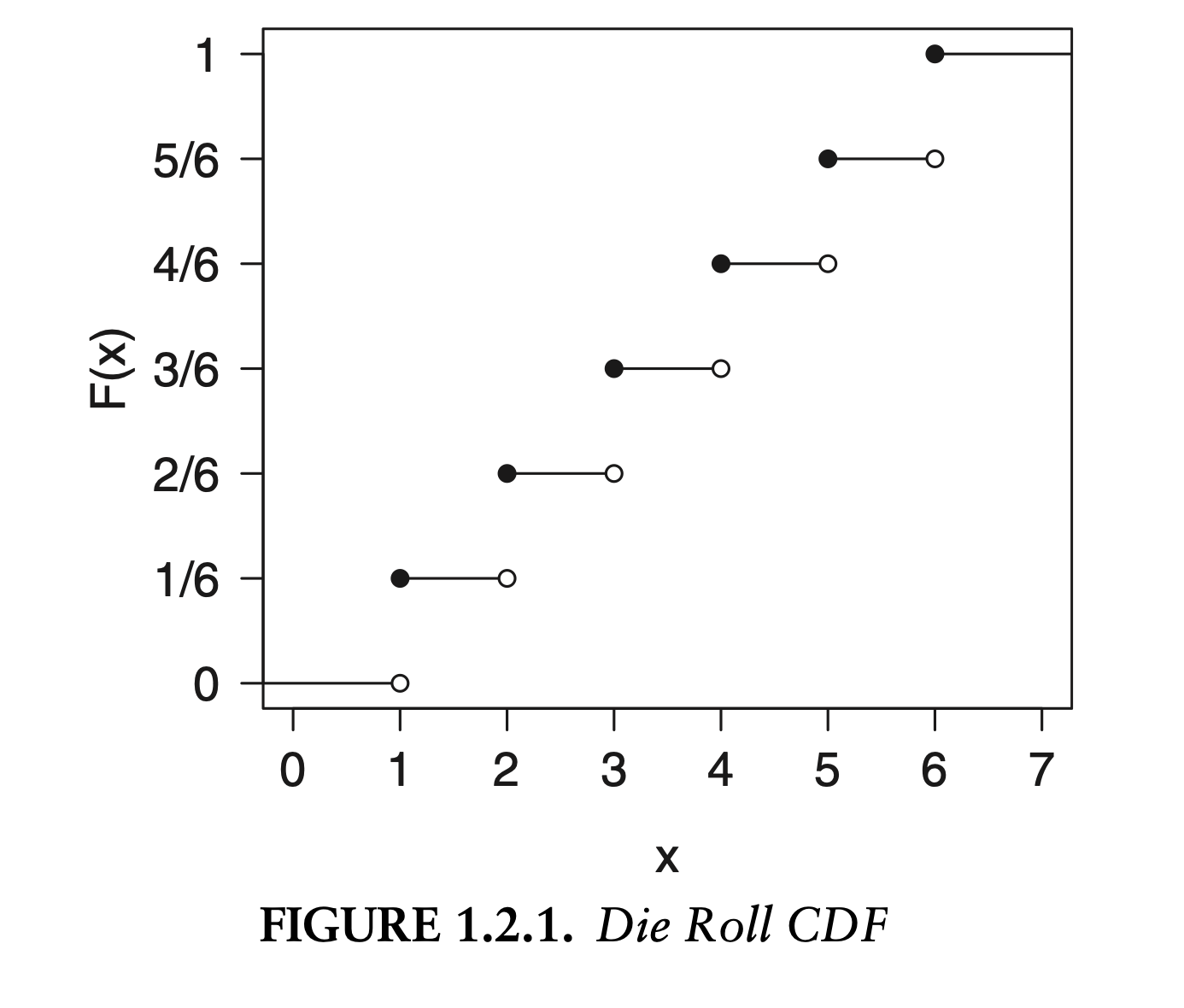
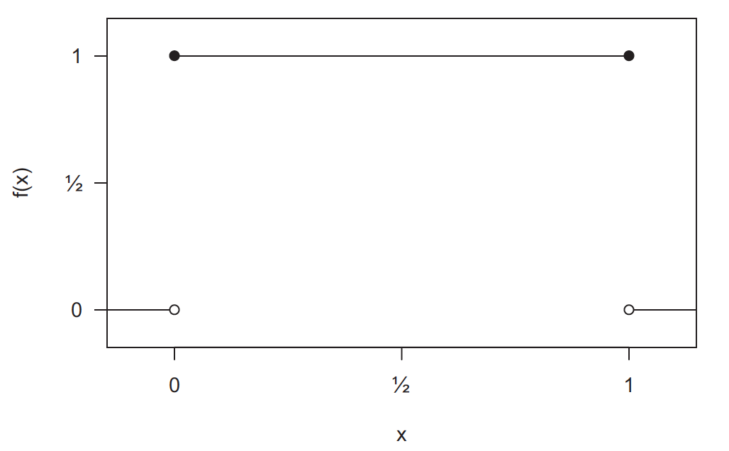
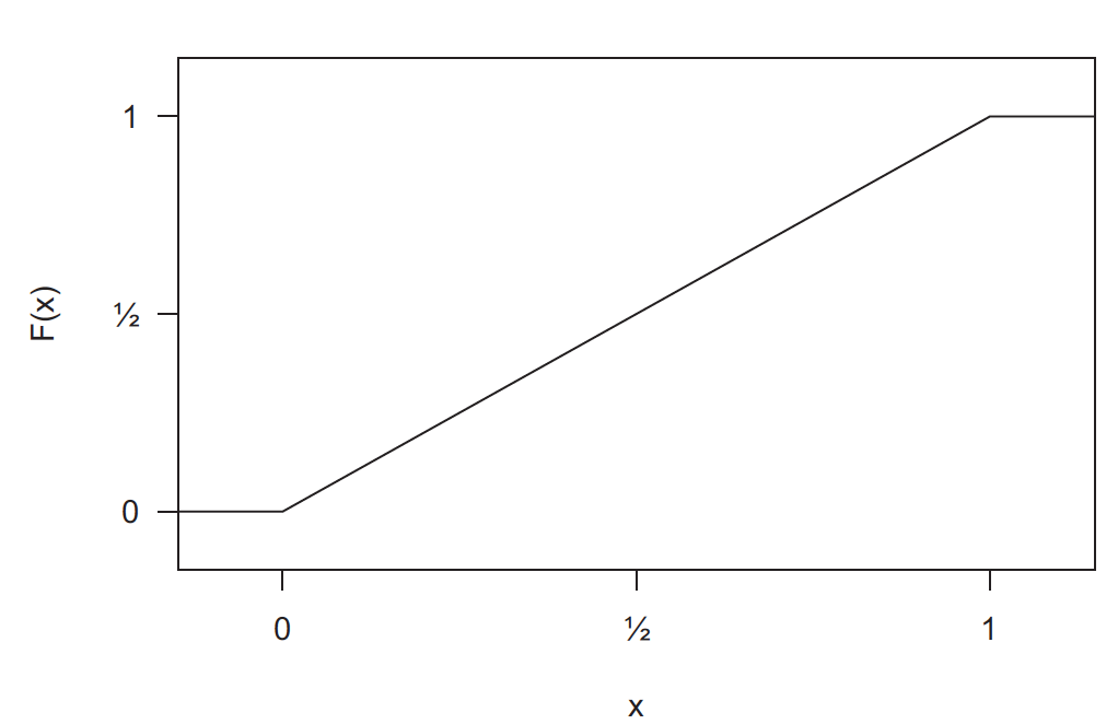
Example: Uniform distribution

Uniform PDF

Uniform CDF

Standard normal distribution

Standard Normal PDF

Standard Normal CDF

Wrapping up

Random variables as useful placeholders to think about properties of data without looking at data

Everything applies to bivariate, multivariate distributions, the math is just messier

Next week: Summarizing random variables to identify ideal quantities that we will try to approximate with data

Aside: distributions in R

d is for density (PMF/PDF)

dbinom(x = 1, size = 1, prob = 0.3)

[1] 0.3

p is for probability distribution function (CDF)

pbinom(q = 0.2, size = 1, prob = 0.3)

[1] 0.7

q is for quantile (inverse CDF)

qbinom(p = 1, size = 1, prob = 0.3)

[1] 1

r is for random number generation

set.seed(123)
rbinom(n = 10, size = 1, prob = 0.3)

 [1] 0 1 0 1 1 0 0 1 0 0