Summarizing Distributions

POLI_SCI 403: Probability and Statistics

Agenda

• Revisit random variables
• Summarizing random variables
• Lab

Last week

In your own words, what is a random variable?

• Discrete random variables have a PMF

• Continuous random variables have a PDF

In either case, they are just functions:

\[ f(x) = Pr[X = x] \]

They important part is that we can operate on them, meaning we can theorize about producing single number summaries that describe them

Expected value

Discrete:

\[ E[X] = \sum_x x f(x) \]

 

Continuous:

\[ E[X] = \int_{-\infty}^{+\infty} xf(x)dx \]

Expected value

Discrete:

\[ E[X] = \sum_x x f(x) \]

 

Continuous:

\[ E[X] = \int_{-\infty}^{+\infty} xf(x)dx \]

These are just weighted averages of each value and its corresponding probability

Why do we like the expected value?

We said a function applied to a random variable yields a random variable

But an operator of a random variable can be treated as a constant

So we can think of them as (theoretical) one-number summaries of a random variable

Rules of expectations

1. If \(a\) is a constant, then \(E[a] = a\)

2. Extension: \(E[aX] = a E[X]\)

3. \(E[X_1 + \ldots + X_p] = E[X_1] + \ldots + E[X_p]\)

Expectations of summations are summations of expectations (ESSE)

Rules of expectations

1. If \(a\) is a constant, then \(E[a] = a\)

2. Extension: \(E[aX] = a E[X]\)

3. ESSE: \(E[X_1 + \ldots + X_p] = E[X_1] + \ldots + E[X_p]\)

4. \(E[b_1X_1 + \ldots + b_pX_p] = b_1E[X_1] + \ldots + b_pE[X_p]\)

Expectations of weighted summations are summations of weighted expectations (EWSSWE)

Rules of expectations

1. If \(a\) is a constant, then \(E[a] = a\)

2. Extension: \(E[aX] = a E[X]\)

3. ESSE: \(E[X_1 + \ldots + X_p] = E[X_1] + \ldots + E[X_p]\)

4. EWSSWE: \(E[b_1X_1 + \ldots + b_pX_p] = b_1E[X_1] + \ldots + b_pE[X_p]\)

• #3 and #4 are true even if random variables are not independent

• These rules make up a very important property

Linearity of expectations

Let \(X\) and \(Y\) be random variables, then \(\forall a, b, c \in \mathbb{R}\)

\[ E[aX + bY + c] = a E[X] + bE[Y] + c \]

Implication: Expected value is a linear operator

Meaning we can rearrange terms for easier calculation

For other things, linearity is not true unless you are explicitly told otherwise

This holds for discrete random variables with joint PMF \(f\), jointly continuous random variables with joint PDF \(f\), and for X discrete and Y continuous or the other way around (but math is cumbersome)

More generally

We can describe a random variable by its moments

\(\mu'_j = E[X^j]\) is the \(j\)th raw moment

So \(E[X] = E[X^1] = \mu'_1\) is the first raw moment

The concept of moment is borrowed from physics. As in torque being the moment of a force.

More generally

\(\mu'_j = E[X^j]\) is the \(j\)th raw moment

Raw moments describe “location”

Sometimes we also want to characterize “spread”, independent from the expected value

\[ \mu_j = E[(X - E[X])^j] \]

is the \(j\)th central moment

Because they convey spread centered in the expected value

The existence of arbitrary moments is important because there is an estimation technique called the method of moments that we do not cover in the sequence.

Central moments

The first central moment is

\[E[X-E[X]]\]

Central moments

The first central moment is

\[E[X-E[X]] \\ = E[X] - E[X]\]

Central moments

The first central moment is

\[E[X-E[X]] \\ = E[X] - E[X] \\ = 0\]

Which is not very useful

Central moments

The second central moment is

\[ E[(X - E[X])^2] \]

Central moments

The second central moment is

\[ E[(X - E[X])^2] \]

Which is called variance

Central moments

The second central moment is

\[ V[X] = E[(X - E[X])^2] \]

Which is called variance

Rearrange to something more applicable:

\[ V[X] = E[X^2] - E[X]^2 \]

Variance is the squared deviation from the expected value

Central moments

The second central moment is

\[ V[X] = E[(X - E[X])^2] \]

Which is called variance

Rearrange to something more applicable:

\[ V[X] = E[X^2] - E[X]^2 \]

The proof here is brief and interesting because it involves treating \(E[X]\) as a constant (cf. Theorem 2.1.13 p. 52)

Why do we stop at the second central moment?

Other central moments are conceptually distinct but not as important for social science applications (more in the lab)

Variance is expressed in squared terms, but if you take the square root you get a measure in units of \(X\)

\[\sigma[X] = \sqrt{V[X]}\]

Which is called the standard deviation

Joint distributions

Sometimes what we want to convey is the relationship between two random variables.

Joint distributions

We can generalize the formula for variance to the bivariate case, which gives the covariance

\[ \text{Cov}[X,Y] = E[(X-E[X])(Y-E[Y])] \]

Alternative formula

\[ \text{Cov}{[X,Y]} = E[XY] - E[X]E[Y] \]

Joint distributions

We can generalize the formula for variance to the bivariate case, which gives the covariance

\[ \text{Cov}[X,Y] = E[(X-E[X])(Y-E[Y])] \]

Alternative formula

\[ \text{Cov}{[X,Y]} = E[XY] - E[X]E[Y] \]

The first formula is helpful to see the connection with centered distances. The second is easier to compute.

Why do we like the covariance?

1. It conveys how much \(X\) and \(Y\) travel together

• Positive: \(\uparrow X \Rightarrow \uparrow Y\)
• Negative: \(\uparrow X \Rightarrow \downarrow Y\)

Correlation is rescaled covariance (0 to 1)

\[ \rho[X,Y] = \frac{\text{Cov}[X,Y]}{\sigma[X] \sigma[Y]} \]

BTW, regression coefficients are also a kind of rescaled covariance.

Aside: Rank correlation

\(\rho\) is Pearson’s correlation

\[ \rho[X,Y] = \frac{\text{Cov}[X,Y]}{\sigma[X] \sigma[Y]} \]

Spearman’s

\[ r_s = \rho[R[X], R[Y]] = \frac{\text{Cov}[R[X],R[Y]}{\sigma[R[X]] \sigma[R[Y]]} \]

Aside: Rank correlation

Kendall’s

\[ \tau = \frac{(\text{# concordant pairs}) - (\text{# discordant pairs})} {(\text{# total pairs})} \]

• concordant: \(x_i > x_j\) and \(y_i > y_j\) OR \(x_i < x_j\) and \(y_i < y_j\)

• discordant otherwise

Aside: Correlation in R

cor(x, y, method = "pearson") # default

cor(x, y, method = "spearman")

cor(x, y, method = "kendall")

Why do we like the covariance?

1. It conveys how much \(X\) and \(Y\) travel together

2. It reminds us that the variance is NOT a linear operator

Variance rule

\[V[X+Y] = V[X] + \color{purple}{2\text{Cov}[X,Y]} + V[Y]\]

Unless \(\color{purple}{\text{Cov}[X,Y]} = 0\)

Meaning?

Independence

What does it mean for \(X\) and \(Y\) to be independent?

Knowing the outcome of one random variable provides no information about the probability of any outcome for the other.

Consequences of independence

• \(E[XY] = E[X] E[Y]\)
• \(\text{Cov} [X,Y] = 0\)
• \(V[X+Y] =V[X] + V[Y]\)

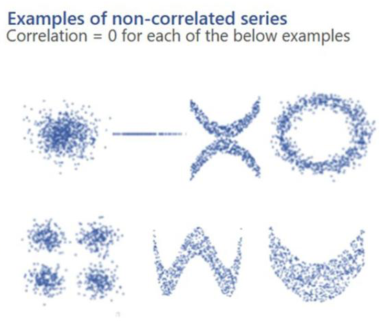
\(\rho [X,Y] = 0\) does not imply independence!

Why?

Distance correlation is a fancier measure that is zero only if two vectors are independent.

Measuring fit

Central moments are centered around the expected value

Example:

\[ V[X] = E[(X - E[X])^2] \]

But we can technically center them on anything we want to

Measuring fit

\[ E[(X-\color{purple}c)^2] \]

Measuring fit

\[ E[(X-\color{purple}c)^2] \]

This is called the

Measuring fit

\[ E[(X-\color{purple}c)^2] \]

This is called the Mean

Measuring fit

\[ E[(X-\color{purple}c)^2] \]

This is called the Mean Squared

Measuring fit

\[ E[(X-\color{purple}c)^2] \]

This is called the Mean Squared Error

Measuring fit

\[ E[(X-\color{purple}c)^2] \]

This is called the Mean Squared Error around \(\color{purple}{c}\)

\(\color{purple}c\) is for cookie constant

Measuring fit

\[ MSE = E[(X-\color{purple}c)^2] \]

Plugging \(\color{purple}{c = E[X]}\) minimizes MSE (cf. Theorems 2.1.23 and 2.1.24)

That’s because you can rearrange to

\[ E[(X-\color{purple}c)^2] = V[X] + (E[X]-\color{purple}c)^2 \]

Eventually, \(c\) will become something more meaningful

Measuring fit

\[ MSE = E[(X-\color{purple}c)^2] \]

Plugging \(\color{purple}{c = E[X]}\) minimizes MSE (cf. Theorems 2.1.23 and 2.1.24)

That’s because you can rearrange to

\[ E[(X-\color{purple}{E[X]})^2] = V[X] + (E[X]-\color{purple}{E[X]})^2 \]

\[ = V[X] \]

The implication is that the expected value is generally a good single-number prediction for what \(X\) will look like

Best predictor

We can say that \(E[X]\) is the best predictor of \(X\) because it minimizes the MSE

This also extends to conditional expectation functions (CEF)

CEF \(E[Y|X]\) minimizes MSE of \(Y\) given \(X\)

 

Wait hold on

Conditional expectation function

Discrete:

\[ E[Y|X=x] = \sum_yyf_{Y|X}(y|x) \]

Continuous:

\[ E[Y|X=x] = \int_{-\infty}^{+\infty}yf_{Y|X}(y|x)dy \]

This is the conditional expectation of \(Y\) given \(X=x\). It looks like an operator but it is actually a function \(G_Y(x)\) (technically, it is composed of many functions)

Conditional expectation function

Note that we can also have

\[ G_Y(X) = E[Y|X=X] = E[Y|X] \]

To denote the random variable that results from applying the CEF (which is technically many functions) to \(X\)

We can just move on with calling \(E[Y|X]\) the CEF

Properties of conditional expectations

• Linearity (same as with unconditional expectations)

Properties of conditional expectations

• Linearity (same as with unconditional expectations)

• Law of Iterated Expectations:\(E[Y] = E[E[Y|X]]\)

Unconditional expectation can be represented as a weighted average of conditional expectations

Properties of conditional expectations

• Linearity (same as with unconditional expectations)

• Law of Iterated Expectations:\(E[Y] = E[E[Y|X]]\)

• Law of Total Variance:

\[ V[Y] = \underbrace{E[V[Y|X]]}_\text{Avg variability within X} + \underbrace{V[E[Y|X]]}_\text{Variability across X} \]

We can decompose the variability in random variable \(Y\) into the variability “within” and “across” values of \(X\)

Best linear predictor

CEF \(E[Y|X]\) minimizes MSE of \(Y\) given \(X\)

If we restrict ourselves to a linear functional form \(Y = a + bX\)

Then the following minimizes MSE of \(Y\) given \(X\):

• \(g(X) = \alpha + \beta X\) where
• \(\alpha = E[Y] - \frac{\text{Cov}[X,Y]}{V[X]}E[X]\)
• \(\beta = \frac{\text{Cov}[X,Y]}{V[X]}\)

For now, just remember this will become very important. The important part is that it can be useful to impose a linear form to the best predictor.

Wrapping up

Do you need to memorize these properties?

No, but a lot of the theory behind fancy methods relies on playing with the properties of expected values/moments of random variables

Down the line: Averages (and average-like things) have statistical properties that make them good one-number summaries (most of the time)

You need a strong case to not use means or conditional means