Unsupervised Learning
POLI_SCI 490
Plan for today
Discussion
- Unsupervised learning
- Clustering
- Principal components
- Extension: Mixture models
- Semi-supervised learning (if we have time)
- Application readings
Unsupervised Learning
Big picture
Why is it called unsupervised?
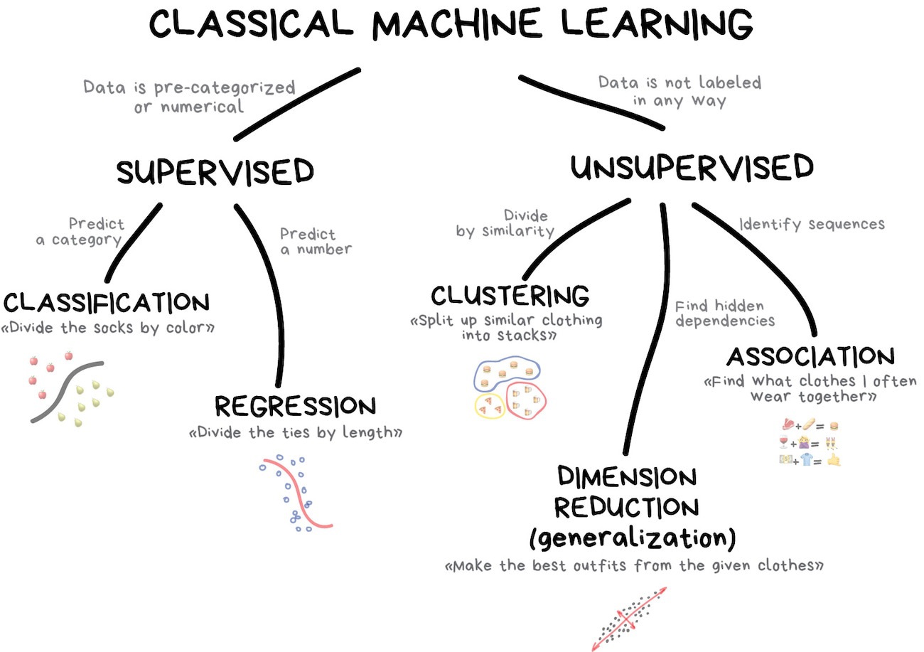
Types
Clustering
Dimension reduction
Types
Clustering \(\rightarrow\) Discrete groups
Dimension reduction
Types
Clustering \(\rightarrow\) Discrete groups
Dimension reduction \(\rightarrow\) Probabilistic membership
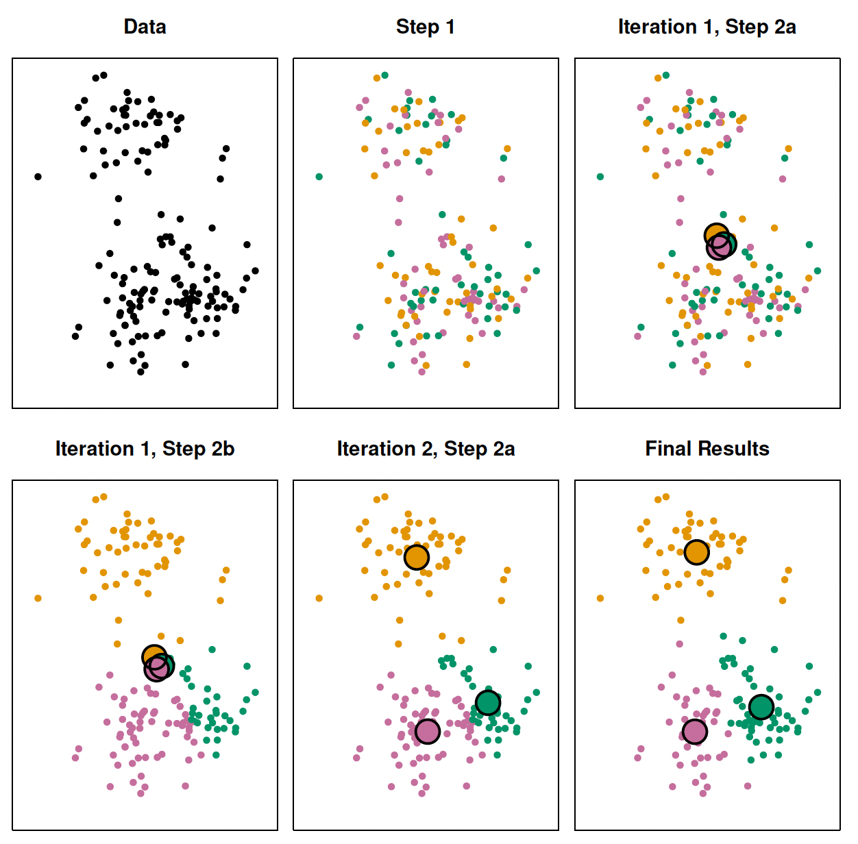
K-means clustering
Algorithm
Randomly assign a number (cluster), from \(1\) to \(K\), to each observation.
Iterate until cluster assignment stops changing:
- For each cluster, compute centroid
- Assign each observation to closest centroid
Stop when within-cluster variation is minimized
\[ \sum_{k=1}^K \text{WCV} (C_k) \]
Considerations
Need to know how many clusters in advance
Clusters are non-overlapping
Every observation must belong to a cluster
Categorical predictors need special handling (see k-medoids clustering)
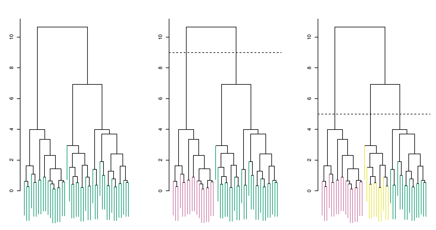
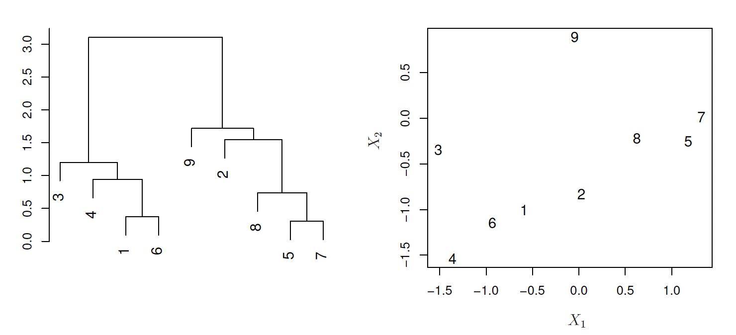
Hierarchical clustering
Algorithm
Assign \(n\) observations to \(n\) unique clusters
Compute pairwise (Euclidean) distances
Fuse two clusters based on distance to compute \(n-1\) clusters
Repeat until all observations belong to a cluster
Which produces a dendrogram
Problem
Combining two observations based on distance is easy
But how do we aggregate based on distances between clusters?
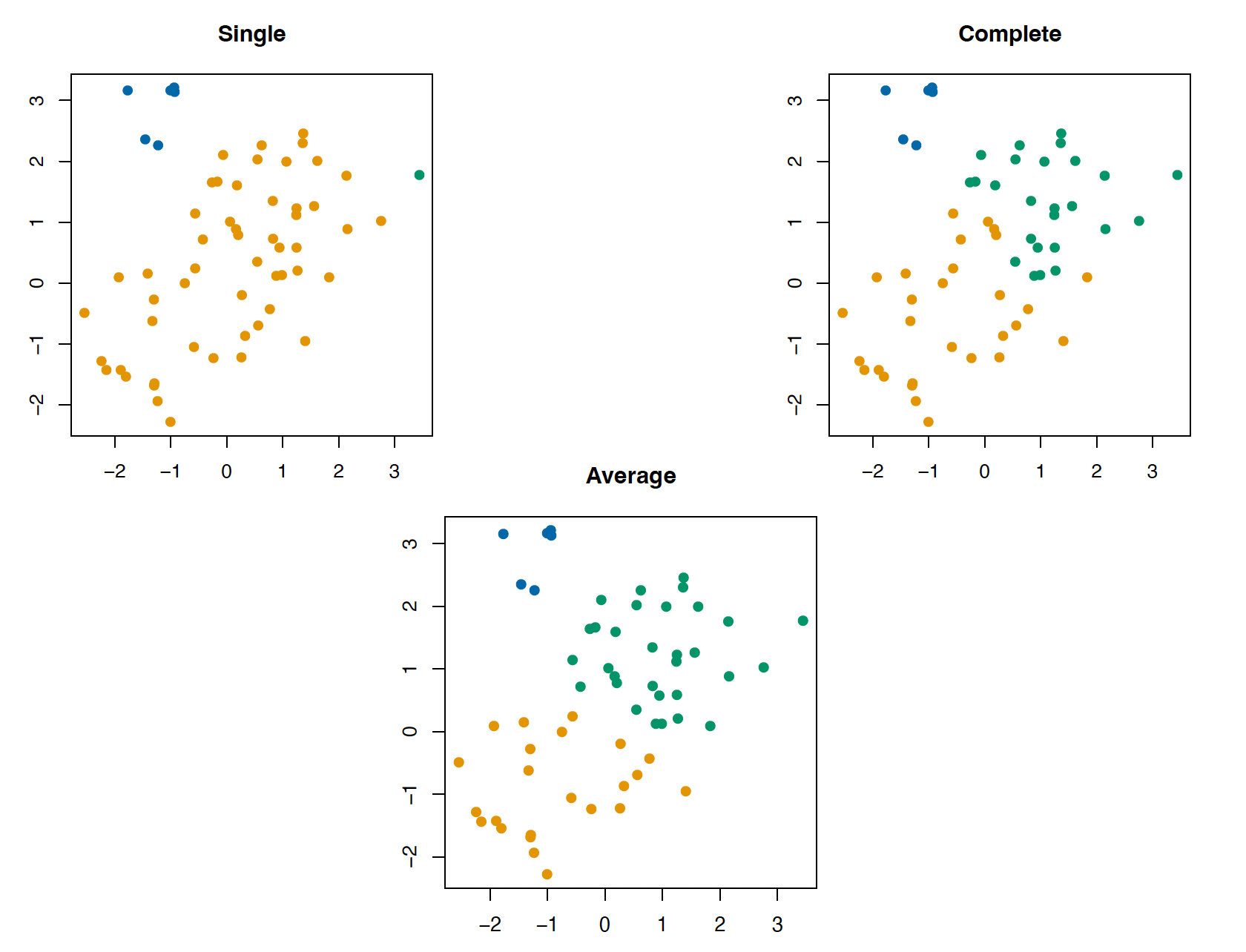
Types of linkage
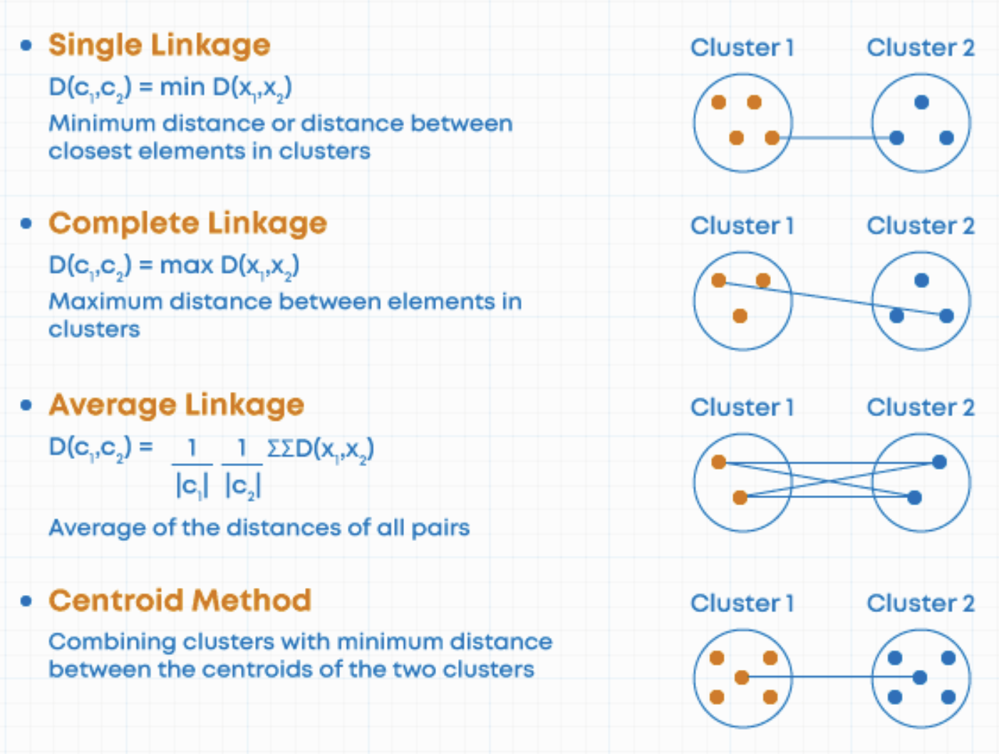
Which linkage to use?
Single linkage suffers from chaining (clusters spread out and not compact enough)
Complete linkage suffers from crowding (clusters are compact but not far enough apart)
Average linkage uses more information, so it balances out
Which linkage to use?
But average linkage suffers from what affects all averages
Outliers
Distance transformations (e.g. squared vs. absolute distance)
Centroids are less sensitive to these issues, but they are not meaningful in some applications
Considerations
No need to pre-specify number of clusters, but need to commit to a cutoff after fitting
Choice of linkage and distance metric is consequential
Every observation must belong to a cluster
Principal components analysis (PCA)
Motivation
We want to visualize \(n\) observations over \(p\) features
That means \(\binom{p}{2}\) possible scatterplots
We want to find a low dimensional representation of the data that captures as much information as possible
Fitting PCA
The first principal \(z_{i1}\) component is a linear combination
\[ z_{i1} = \phi_{11}{x_{i1}} + \phi_{21}{x_{i2}} + \ldots + \phi_{p1} x_{ip} \]
The \(\phi\) elements are a vector of factor loadings
Like a map to convert the values across \(p\) predictors into one dimensional space
Fitting PCA
We find the values of \(\phi\) by optimizing
\[ \underset{\phi_{11}, \ldots, \phi_{p1}}{\text{maximize}} \left \{ \frac{1}{n} \sum_{i=1}^n \left (\sum_{j=1}^p \phi_{j1} x_{ij} \right )\right\} \text{ subject to } \sum_{j=1}^p \phi_{j1}^2 = 1 \]
Meaning we are looking for factor loadings that maximize sample variance
The second principal component is is fitted in the same way, except that we constrain it to the set of linear combinations that are uncorrelated (orthogonal) to the first component
Another way to think about it
The first principal component loading vector is the line in \(p\)-dimensional space that is closest to the \(n\) observations
Adding the second, we make a plane
and the third to make a hyperplane
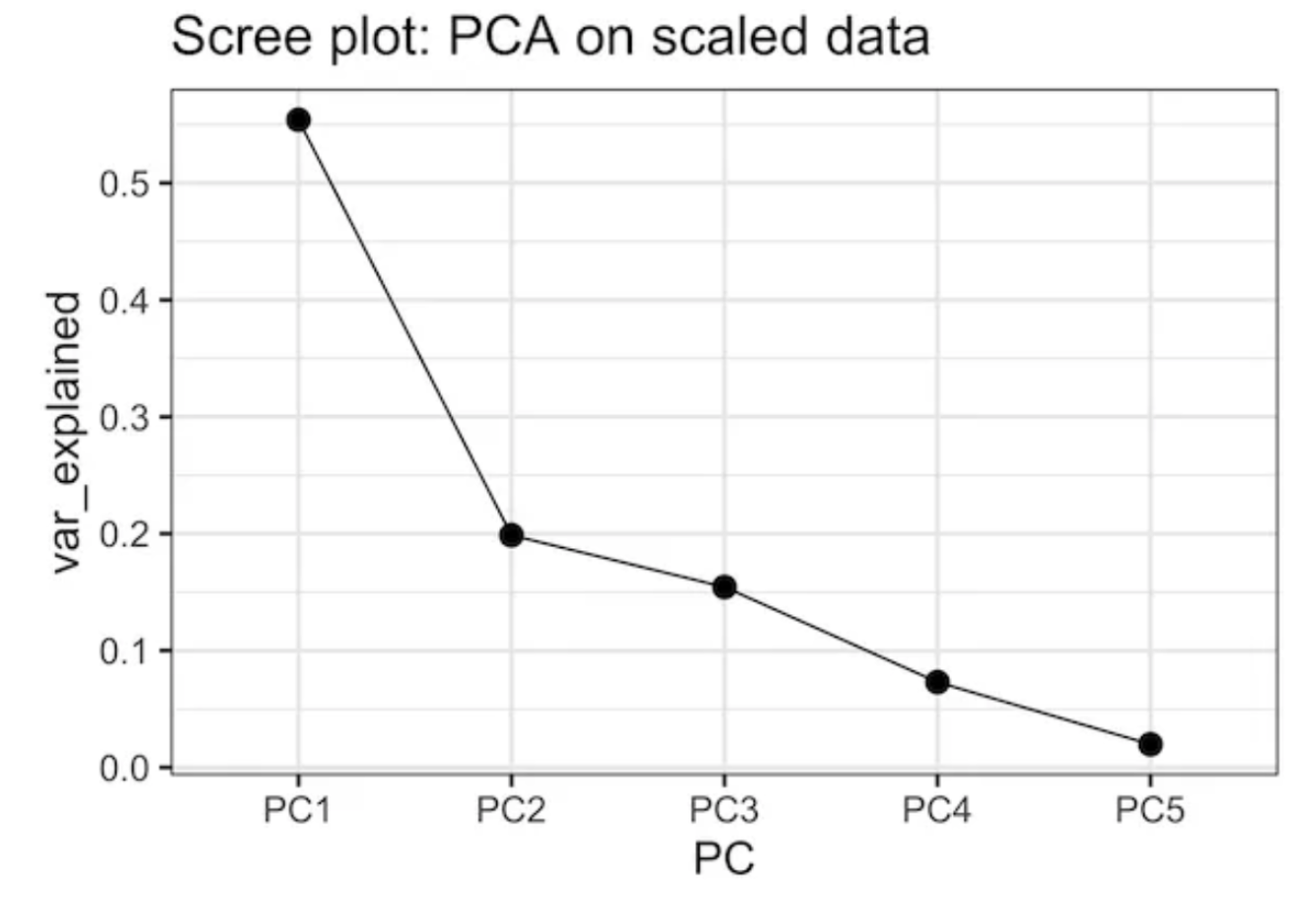
Proportion of variance explained
The main idea is to reduce dimensions without dropping much information
We can determine the proportion of variance explained by a given number of principal components
\[ \text{PVE} = 1 - \frac{\text{RSS}}{\text{TSE}} \]
Which also helps us to determine how many components are relevant to characterize the data
We can interpret the values of \(z_{im}\) as measures of how much an observation belongs to that component
Considerations
PCs are more abstract than clusters
Choice of relevant dimensions is arbitrary
Restricted to linear combinations (but see ESL on principal curves and surfaces)
Needs complete data set
Extension
So far
We have unsupervised learning algorithms that either:
Make discrete clusters that drop information
Assign scores but are too restrictive and hard to interpret
Surprise! The solution is to take a Bayesian approach
Mixture models
A family of Bayesian models that aims to identify subgroups within a population
The key is to assume that the data is generated by a multimodal distribution, then we can estimate posterior probabilities for each unit belonging to a group
Example 1
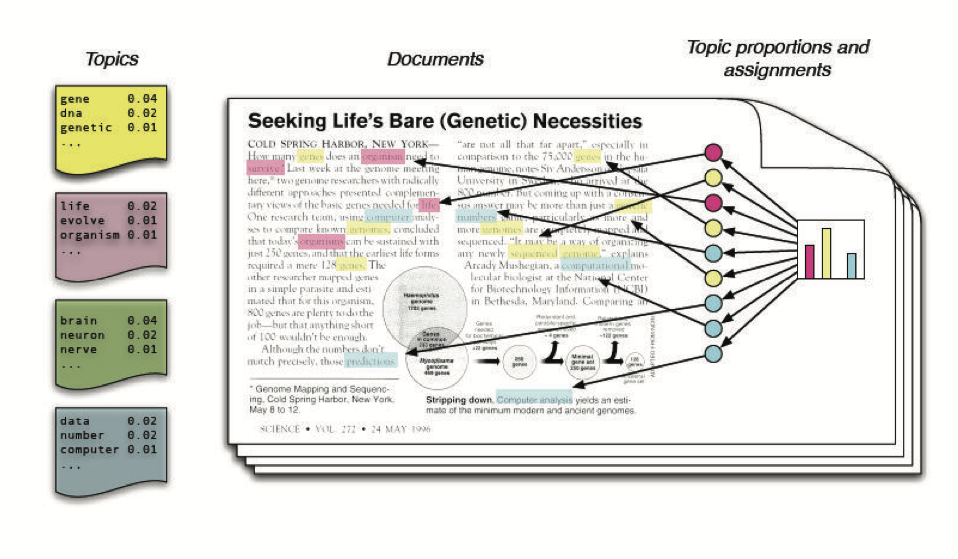
Latent Dirichlet Allocation (LDA)
LDA
Motivation: Latent topics in a document have a lot of in-betweenness
Considerations
We get both topic proportions and assignments
Need to choose and validate the number of topics
Does not read between the lines (but see STM)
Example 2
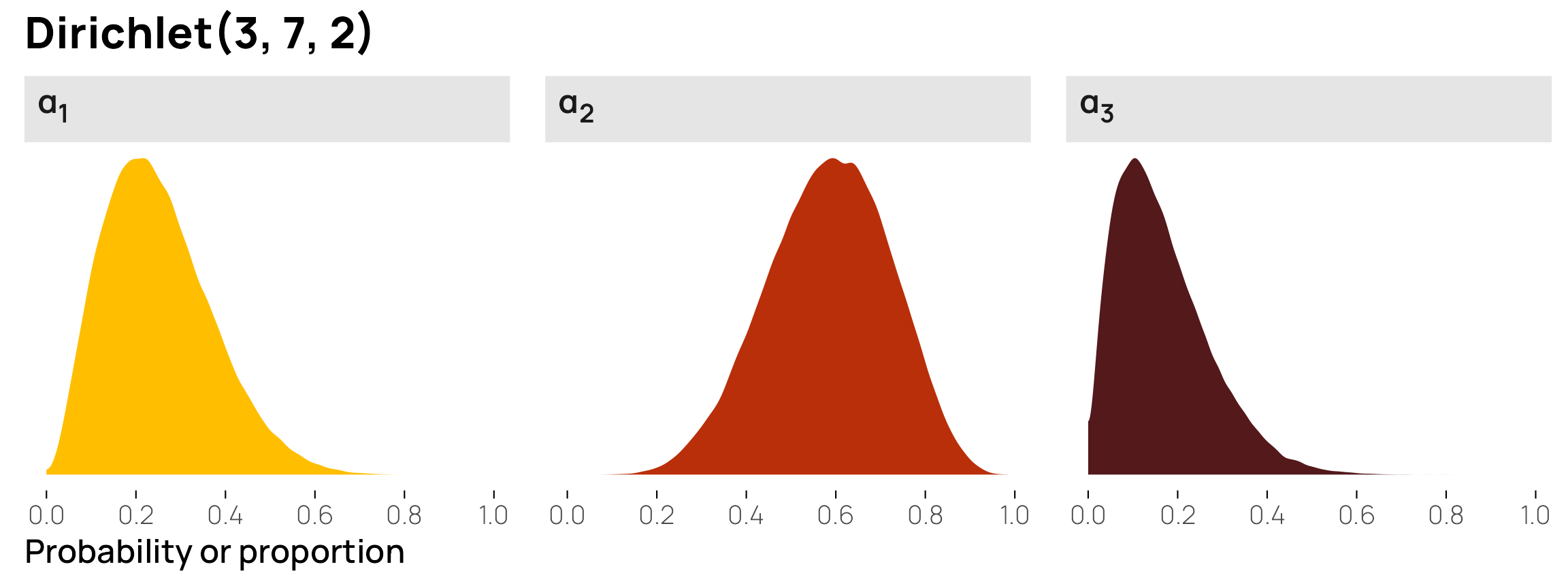
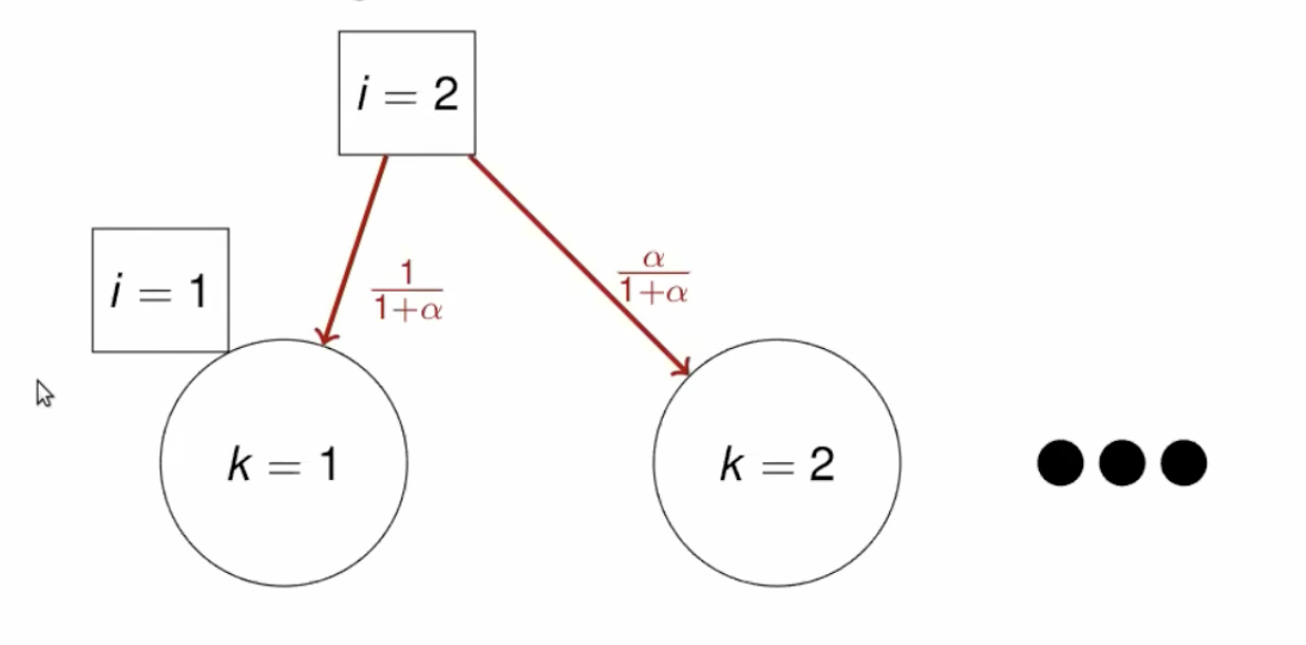
Chinese Restaurant Proces (CRP)
CRP
Motivation: Seating customers in a restaurant with infinite tables of infinite capacity each
Start with a customer seating in one table
A new customer is assigned to a new table with probability \(\frac{\alpha}{(i-1)+ \alpha}\)
and to an existing table with probability \(\frac{n_k}{(i-1)+ \alpha}\)
where \(n_k\) is the number of customers at a table and \(\alpha\) is a concentration parameter
Larger \(i\) \(\rightarrow\) smaller probability of new cluster
Whiteboard
Considerations
LDA and topic models are finite mixture models
CRP and alike are nonparametric mixture models
CRP models a “rich get richer” process
Creates fewer clusters
Still need to choose a parameter
Computationally intensive
Overall
Unsupervised learning is an impressionistic endeavor
No matter what you do, you need to defend your choice of hyperparameters
Bonus-track
Semi-supervised learning
Motivation
What do you do if you do not have labels for supervised learning?
Annotate a human-scale proportion of observations
Use them as a training set to then predict the rest of the data
If you do too little, you may overfit on the training data
Doing enough may take forever!
Alternative: SSL
Label some data
Use an unsupervised learning algorithm to learn structure in both labeled and unlabeled data
Train supervised learning algorithm on the extended data
Evaluate test performance
We reduce overfitting but lose (potential) precision
Approaches to SSL
Cluster-then-label: Assume observations in the same cluster should have same label
Wrapper methods: Create probabilistic pseudo-labels, retain high certainty observations and retrain (smoothness assumption)
Active learning: Use unsupervised algorithm to determine which observations should be manually labeled next